Heat Equation with Two Spatial Variables
After completing my project called heat-wave-equation-simulator, which is a project for simulating the heat equation, wave equation and wave equation with damping using one spatial variable, I was inspired to extend the concept to two spatial variables, leading to the development of this heat simulation project. This project explores numerical methods and visualization techniques to model heat distribution dynamically across a given area.
For more information and to explore the codebase, please refer to the GitHub repository.

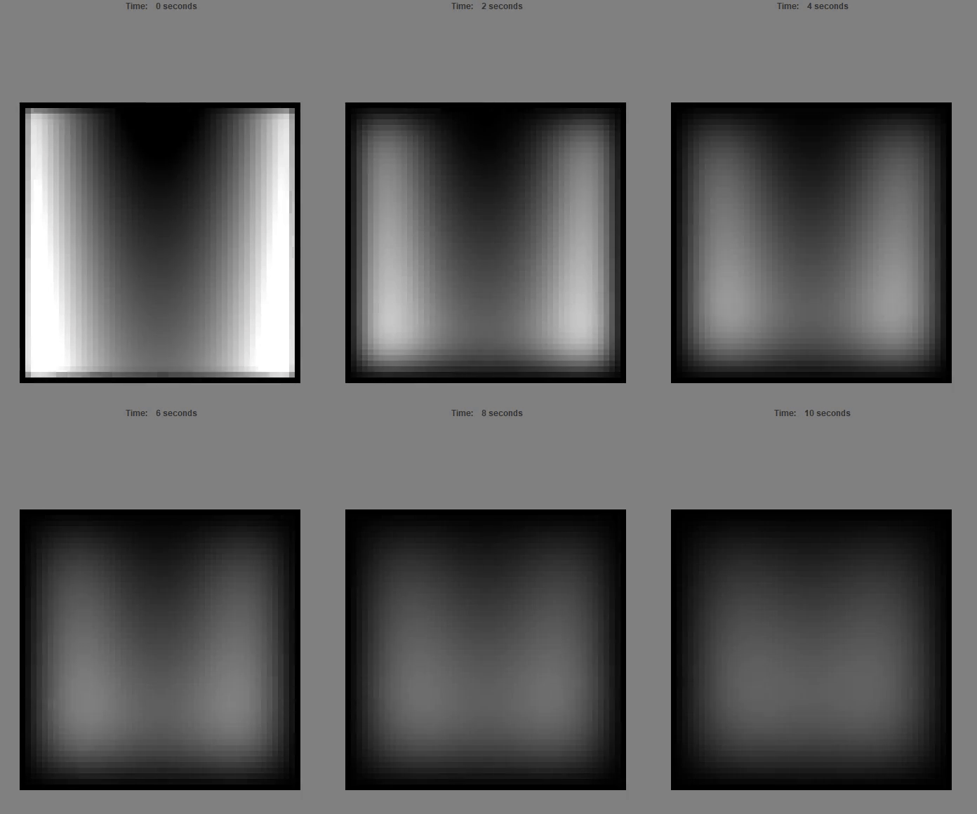
Heat Diffusion: Over time, the temperature diffuses throughout the medium due to the lower temperature of the boundary, which is permanently set to zero.
Project Overview
The heat simulation project is designed to model the distribution of heat across a square domain over time, using the finite difference method to solve the 2D heat equation numerically. The boundary conditions are set to zero, and the initial heat distribution is represented by a polynomial spline surface constructed by utilizing Hermite spline interpolation. The points used to construct the polynomial spline are from user-defined input points in 3D space.
Key Components
The project is structured around several core components.
- Numerical Solution Logic (
NumericalSolution.java): This part of the project contains the algorithms and methods used to compute the heat distribution. It involves complex mathematical computations and iterative processes to simulate heat flow accurately. The finite difference method is implemented to approximate the heat equation, while Hermite spline interpolation constructs the initial heat distribution. - Main Control Program (
MainHeat.java): This is the central part of the project, responsible for setting up the simulation environment, initializing variables, and handling user inputs. It acts as the coordinator, ensuring that all components work together. Users can adjust settings such as the thermal diffusion constant, time step, and mesh size for the square grid inMainHeat.java. - Simulation Execution (
HeatSimulation.java): This component runs the actual simulation, updating the heat distribution over time and displaying the results. It handles the graphical representation and allows for visualization of the simulation progress.
Code Overview
In this section we will highlight the essential parts of the code to the previously mentioned scripts.
NumericalSolution.java Script
The method called updateVelocity() updates the temperature change (velocity) using the finite difference method. It sets up a linear system to calculate temperature changes and updates the dataMatrix to simulate heat distribution over time.
public void updateVelocity(double deltaTime) {
// Setup matrix sizes
int rowSize = dataMatrix.getNumRows();
int colSize = dataMatrix.getNumCols();

// Create linear system Ax = b
double[][] linSys = new double[size][size];
double[][] vectorData = new double[size][1];

// Finite difference calculations (pseudocode)
for each interior point (i, j) {
    calculate change in temperature using neighbors;
}

// Update temperatures
for each interior point (i, j) {
    dataMatrix[i][j] += velocityMatrix[i][j] * deltaTime;
}
}
MainHeat.java Script
This code snippet sets up the simulation environment with user-defined points, thermal diffusion constant called 'alpha', and mesh size. It creates a HeatSimulation object and runs the simulation, continuously updating the heat distribution.
public class MainHeat {
public static void main(String[] args) {
    // Initialize user-defined points
    List points = new ArrayList<>();
    points.add(new Vertex(1, 2, 3));
    points.add(new Vertex(4, 5, 6));

    // Set simulation parameters
    double alpha = 0.01;
    int meshX = 50;
    int meshY = 50;

    // Setup simulation
    HeatSimulation simulation = new HeatSimulation();
    NumericalSolution solution = simulation.setupSimulation(points, alpha, meshX, meshY);

    // Simulation loop
    while (true) {
        solution.updateVelocity(0.1);
        // Visualize results
    }
}
}
HeatSimulation.java Script
The following method called SetupSimulation() sets up the simulation by creating a spline surface from user-defined points and projecting it onto a 2D mesh. The resulting dataMatrix represents the initial heat distribution, which is used to create a NumericalSolution object for the simulation.
Furthermore, the method projectToMesh() constructs a mesh grid using a SimpleMatrix object. Each cell on the grid, consisting of an (\(x\), \(y\)) coordinate, is then evaluated using a Polynomial object which represents the current heat wave solution to obtain the current function value (temperature value).
public class HeatSimulation {
public NumericalSolution setupSimulation(List points, double alpha, int meshX, int meshY) {
    // Create spline surface from points
    Polynomial poly = CreateSplineSurface(points);

    // Project spline onto 2D mesh
    SimpleMatrix dataMatrix = projectToMesh(poly, meshX, meshY);

    // Return numerical solution
    return new NumericalSolution(dataMatrix, alpha);
}

private SimpleMatrix projectToMesh(Polynomial poly, int meshX, int meshY) {
    SimpleMatrix matrix = new SimpleMatrix(meshX, meshY);
    // Fill matrix with projected values (pseudocode)
    for each cell (x, y) in mesh {
        matrix[x][y] = poly.evaluate(x, y);
    }
    return matrix;
}
}
Conclusion
This project bridges theoretical and practical aspects of differential equations, offering a way to visualize and understand heat distributions. By extending the heat-wave-equation-simulator to two spatial variables, it demonstrates the application of numerical methods in simulating differential equation over time. Future improvements could include optimizing calculations for better performance and exploring more complex boundary conditions.
