Optimized Matrix Multiplication Algorithm in C
My first project in learning C focused on creating a custom memory allocator. To further build on my understanding, I chose to implement an optimized matrix multiplication algorithm, further exploring low-level programming, and also learning about multithreading and SIMD vectorization. Matrix multiplication is an ideal choice because it relies on well-written low-level code to optimize memory layout and CPU cache utilization. Additionally, matrix multiplication can be divided into independent sub-tasks which allows for efficient parallelization through multithreading and vectorization.
This project is divided into two parts: an experimental main section and a theoretical appendix. In the experimental part, the focus is on benchmarking various matrix multiplication algorithms and analyzing their performance. Additional emphasis is put on my two top-competing algorithms to determine which is better. Thereafter, all algorithms are compared, including OpenBLAS, an industry-standard library. The theoretical appendix provides explanations of the algorithms developed, starting with the naive implementation and progressively incorporating ideas and concepts such as blocking / tiling, multithreading with POSIX threads, and SIMD vectorization, utilizing the AVX registers on the CPU.
As this is a project focused on the iterative process of optimizing the runtime performance of algorithms, less emphasis has been placed on ensuring that the floating-point accuracy is identical to that of OpenBLAS for all matrix dimensions and element values. Instead, this project operates within well-defined constraints to ensure accuracy within threshold values to that of OpenBLAS. While this approach does not guarantee identical accuracy for all scenarios, it allows for optimization and meaningful comparisons within this framework.
For more information and to explore the codebase, please refer to the GitHub repository.
Project Overview
As mentioned in the introduction, this project is divided into two parts: an experimental section, where benchmarking and analysis are the focus, and a theoretical appendix, which provides detailed explanations of the matrix multiplication algorithms developed, including naive, blocking, multithreading and AVX-optimized implementations. For future reference, each name for the algorithms developed is included in the section titles of the appendix, as outlined below in the Theoretical Background Overview. This way, readers can find detailed explanations of each algorithm when they encounter these names later in the experiments section.
Experiments Overview
- Benchmarking Framework and Methodology: Discuss the assumptions and benchmarking framework used to ensure consistency and experimental rigor in the analysis.
- Verification Framework: Highlight the framework to test the correctness of the algorithms to that of OpenBLAS.
- Data Collection Approach: Discuss the general framework used for data collection and benchmarking of the implemented algorithms, along with compiler optimization flags.
- Blocking Size Optimization for Competing Algorithms: Determine the optimal blocking size for the two top-performing algorithms.
- Selection of the Best Algorithm: Statistical methods are applied to benchmark data to identify the best-performing algorithm based on mean execution time.
- Benchmarking Algorithms: Benchmarks are conducted on all implemented algorithms, with OpenBLAS serving as the industry standard for insight.
Theoretical Background Overview (Appendix)
- Naive Matrix Multiplication Algorithm -
NAIVE: To establish a foundational understanding of the problem, we begin with the simplest implementation of matrix multiplication. This serves as a baseline for performance and for later algorithms to build upon. - Blocking / Tiling Method -
SINGLETHREAD: Implement the blocking (tiling) method and explore its advantages, and how it improves algorithm efficiency by optimizing memory access patterns. - Multithreading -
MULTITHREAD: Multithreading fundamentals are applied to refactor the algorithm, utilizing parallelism to maximize CPU utilization. - SIMD Vectorization -
MULTITHREAD_3AVX,MULTITHREAD_9AVX: Integrate AVX (Advanced Vector Extensions) to enable vectorized operations, enhancing computational efficiency.
1. Experiments
This section provides an in-depth analysis of the experiments and the performance of the implemented algorithms. The results highlight the performance improvements achieved with each optimization step and compare them against the industry standard, represented by OpenBLAS.
1.1 Verification Framework
To rigorously perform the experiments, a verification framework was first established to ensure the correctness of the algorithms. To guarantee a floating-point accuracy comparable to that of OpenBLAS, the following constraints were set in place.
VALUES_MIN-1e+6: Chosen to ensure values are within a safe range, minimizing the likelihood of floating-point round-off errors during computations.VALUES_MAX1e+6: The upper bound for element values in the matrices, complementingVALUES_MINto establish a safe range.DIMENSION_SIZE2000 x 2000: A size to balance being computationally feasible for the system and large enough to evaluate the performance of the algorithms on sizable matrices.APPROXIMATION_THRESHOLD1e-9: Ensures that the floating-point accuracy of the created algorithms remains comparable to that of OpenBLAS.
A matrix dimension of 2000 x 2000 was used to have an upper bound for the algorithms during benchmarking It is assumed that smaller square matrices of this size will have comparable floating-point accuracy, as they involve fewer multiplications, reducing the likelihood of floating-point precision loss and round-off errors.
For more about verification and correctness, please refer to the source files.
matrix_mult_naive_verification.cmatrix_mult_single_verification.cmatrix_mult_multi_verification.c
1.2 Data Collection Approach
The data collection when performing the experiments is handled in the bash script, run_benchmark.sh. The run_benchmark.sh script automates the benchmarking collection for the algorithms and places the result in benchmark_results.csv. The bash script handles the following.
- Warm-Up Runs: Before collecting data, the script performs warm-up runs to stabilize the system's runtime behavior and ensure consistent CPU cache states to ensure fairness in the comparison.
- Multiple Benchmark Runs: Each algorithm is benchmarked across multiple matrix dimensions:
50 x 50100 x 100200 x 200500 x 500750 x 7501000 x 10001500 x 15002000 x 2000
NUM_RUNS=50independent runs. This allows for accurate averages and variances in performance metrics. - Performance Metrics Collection: The script uses the Linux
perftool to gather key performance metrics during each benchmark run, including:- Execution time (seconds)
- CPU cycles
- Instructions executed
- Cycles per Instruction (CPI)
- Cache misses
- Cache references
- Cache-miss rate
- Statistical Analysis: For each metric, the script calculates the average and sample variance across all runs, providing insights into both performance and variability.
Compiler Optimization Flags: The GNU Compiler Collection (GCC) was used with the following flags to maximize performance.
CFLAGS = -Wall -O3 -mavx -march=native -funroll-loops -fopenmp
-O3: Enables aggressive optimizations, including loop unrolling and inlining.-mavx: Utilizes AVX instructions for SIMD optimizations.-march=native: Optimizes the compiled code for the specific architecture of the target machine.-funroll-loops: Unrolls loops to reduce branching overhead and improve pipeline performance.-fopenmp: Enables OpenMP support for multithreading, allowing efficient utilization of multiple CPU cores.
For the block size optimization of the competing algorithms, the bash script run_block_size_benchmark.sh was used to collect data. The performance metrics remain identical to those mentioned for the algorithm benchmarks, with the key difference being the addition of block size as an extra parameter during data collection. Results for MULTITHREAD_3AVX and MULTITHREAD_9AVX were stored in MULTITHREAD_3AVX_block_size_results.csv and MULTITHREAD_9AVX_block_size_results.csv, respectively.
1.3 Block Size Optimization for Competing Algorithms MULTITHREAD_3AVX and MULTITHREAD_9AVX
In implementing SIMD vectorization using 256-byte AVX registers, two algorithm versions were developed: MULTITHREAD_3AVX and MULTITHREAD_9AVX. The first employs the minimum number of registers required to fully utilize SIMD vectorization for matrix multiplication, while the second scales the use of AVX registers by a factor of three to potentially improve performance. Both algorithms use the same underlying technique, the latter has more AVX registers to work with, which may lead to better performance.
To maximize the performance of each algorithm, having the optimal block size is crucial. This ensures that data loaded into the CPU cache is optimally utilized and minimizes time spent refetching discarded data. An optimal block size reduces overhead from memory latency. Initial exploratory runs provided an indication that block sizes of 64 and 128 tended to perform better on average. However, a systematic benchmark is required to rigorously evaluate block size performance and determine whether these sizes are truly optimal.
In this section, we perform a benchmark of predefined block sizes across the matrix dimensions discussed in Section 1.2. The predefined block sizes are given by
\[ I=\{8, 16, 32, 64, 128, 256\}. \]Powers of two were selected to simplify the search space, and due to their alignment with with cache lines. For each block size, the average execution time is evaluated using heatmaps to visualize trends across dimensions. This allows us to inspect and identify the two most promising block sizes based on mean execution time.
With the two candidate block sizes identified, \(\beta_{1}\) and \(\beta_{2}\), we perform a two-tailed Welch's t-test to evaluate their performance differences. We have the null and alternative hypotheses defined as
\[ H_0: \mu_{\delta,\beta_{1}} = \mu_{\delta,\beta_{2}} \] \[ H_a: \mu_{\delta,\beta_{1}} \neq \mu_{\delta,\beta_{2}} \]
where \(\delta \in I\) represents the dimension, and \(\mu_{\delta,\beta_{j}}\) denotes the average execution time for block size \(\beta_{j}\) at dimension \(\delta\).
Since the test is performed independently for each of the eight dimensions, the initial significance level \(\alpha = 0.05\) must be adjusted to account for the increased risk of Type I errors (false positives) due to multiple comparisons. The cumulative risk arises because performing multiple tests increases the probability of incorrectly rejecting at least one null hypothesis. By applying the Bonferroni correction, the significance level is adjusted to \(\alpha = \frac{0.05}{8} = 0.00625\), reducing the likelihood of Type I errors. However, this conservative approach comes at the cost of an increased risk of Type II errors (false negatives). This happens because the adjusted threshold requires stronger evidence in the data to reject the null hypothesis in favor of the alternative hypothesis.
The systematic approach of applying a two-tailed Welch's t-test ensures a rigorous comparison, allowing us to select the optimal block size for each algorithm. In the subsequent section 1.4, these results will be used to compare MULTITHREAD_3AVX and MULTITHREAD_9AVX to determine the overall better-performing algorithm.
1.3.1 Optimizing Block Size for MULTITHREAD_3AVX
Considering the benchmark data in MULTITHREAD_3AVX_block_size_results.csv, we construct the following heatmap to illustrate how different block sizes affect the execution time for varying matrix dimensions.
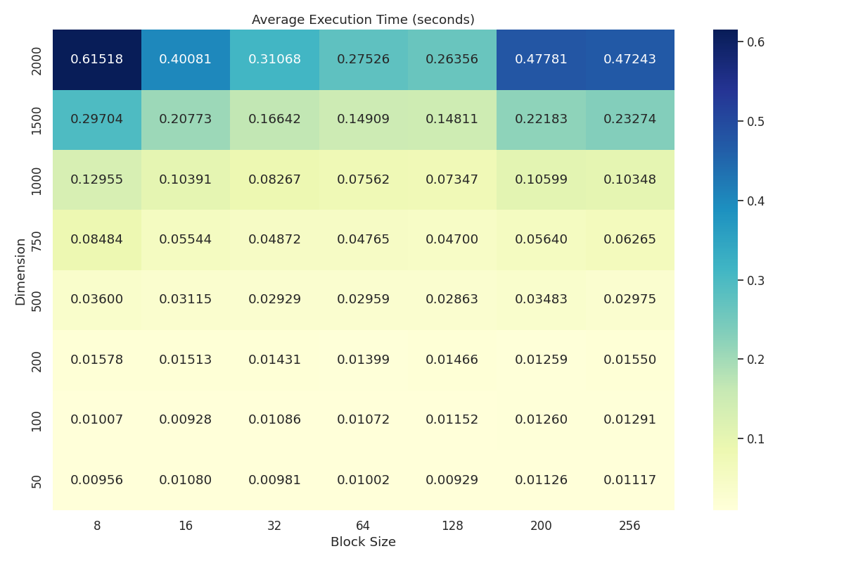
Execution Time Heatmap: Displays average execution time (seconds) with respect to matrix dimensions and block size for MULTITHREAD_3AVX.
Inspecting the heatmap, we observe that block sizes 64 and 128 show better performance compared to the other block sizes for dimensions \(\delta = 2000\) and \(\delta = 1500\). Further observations indicate that these two block sizes also perform relatively well across the lower dimensions. Based on this examination, we select block sizes 64 and 128 for further evaluation using Welch's t-test to determine the better-performing block size among the two.
For transparency, it is important to acknowledge that the understanding of "better performance" in this case is a subjective heuristic. Rather than defining a formal metric or objective function, the selection was based on a simple inspection of the mean execution times. The choice reflects an intuitive assessment that block sizes 64 and 128 tend to perform well for the higher dimensions and relatively well for the lower dimensions compared to the other block sizes.
The results of the two-sided Welch's t-test are visualized in the following plot.
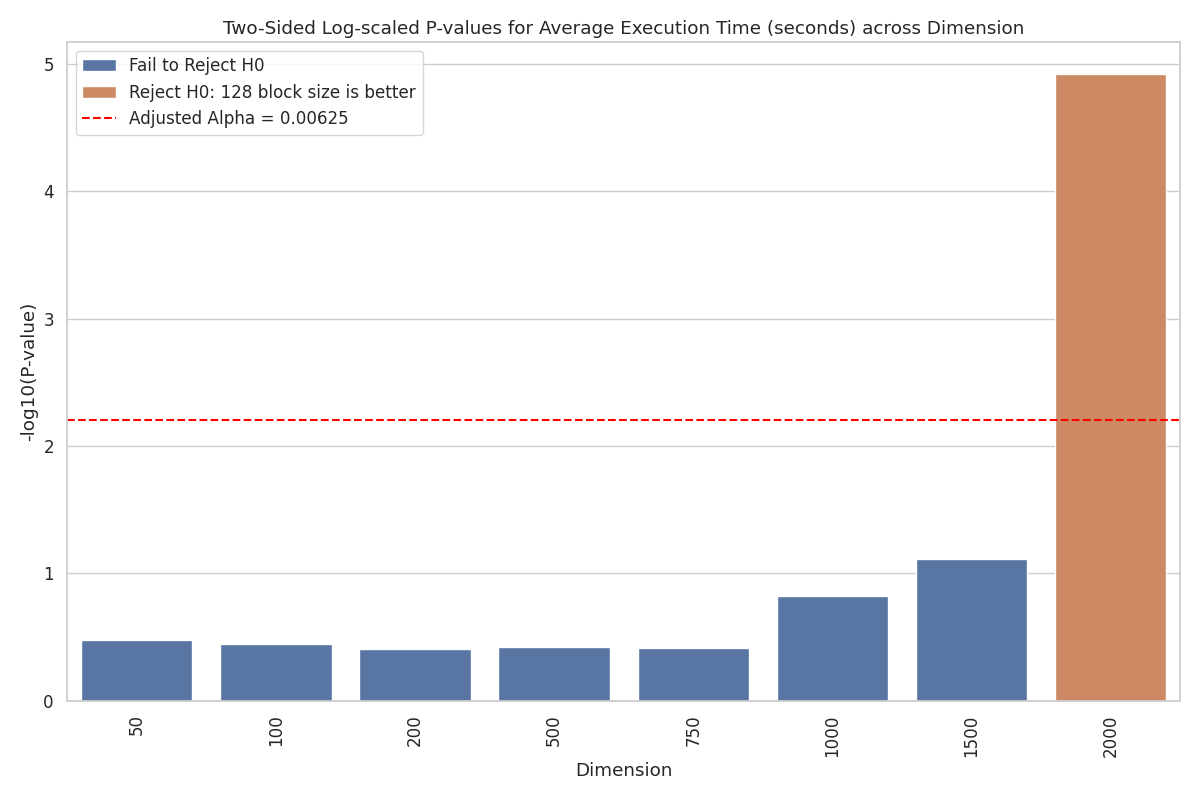
Rejection Threshold Plot: This plot visualizes p-values transformed as \(-\log_{10}(\text{P-value})\) for easier interpretation, and hypothesis rejection outcomes for MULTITHREAD_3AVX across different dimensions. Each bar corresponds to a specific dimension and represents its p-value. The red dotted line marks the adjusted alpha significance threshold (after Bonferroni correction). Brown bars indicates the rejection of \(H_{0}\) and that block size 128 has a smaller mean execution time than block size 64. Blue bars indicate failure to reject \(H_{0}\).
From the plot, we observe a trend where the transformed p-values, given by \(-\log_{10}(\text{P-value})\), increase (implying decreasing untransformed p-values) as the matrix dimension rises, with a rejection of \(H_0\) at \(\delta = 2000\). This rejection strongly supports \(H_a\), indicating that the mean execution times for the two block sizes differ significantly at this dimension. Inspecting the heatmap for \(\delta = 2000\) confirms that block size 128 has a lower mean execution time, supporting the conclusion that it performs better at this dimension. Moreover, the trend of decreasing p-values suggests that as the dimension increases, the performance difference between block sizes 64 and 128 becomes more pronounced. At higher dimensions, block size 128 consistently demonstrates a smaller mean execution time, further highlighting its advantage in these scenarios. However, this interpretation should be approached with caution, as the data shows no significant differences between the two block sizes at lower dimensions. Therefore, at these smaller dimensions, the test results indicate that the data does not provide sufficient evidence to reject \(H_0\), leaving open the possibility that the two block sizes perform similarly under these conditions.
It is important to note that failing to reject \(H_0\) does not imply that \(H_0\) is true. Instead, it reflects insufficient evidence to favor the alternative hypothesis \(H_a\). This could be due to variability in execution times, the sample size, or inherently small differences in performance at smaller dimensions. Additionally, the Bonferroni-adjusted significance threshold of 0.00625 further increases the difficulty of detecting differences, as it requires very strong evidence to reject \(H_0\).
Considering the results across all dimensions, the trend suggests that block size 128 generally outperforms block size 64, particularly for larger matrices where performance differences are more evident. For smaller dimensions, the t-tests do not reveal significant differences, and the data is consistent with both block sizes performing similarly in those cases. Concluding, we therefore select block size 128 as the optimal block size for MULTITHREAD_3AVX.
1.3.2 Optimizing Block Size for MULTITHREAD_9AVX
Using a similar procedure as with MULTITHREAD_3AVX, we analyze the data from MULTITHREAD_9AVX_block_size_results.csv and construct a heatmap.
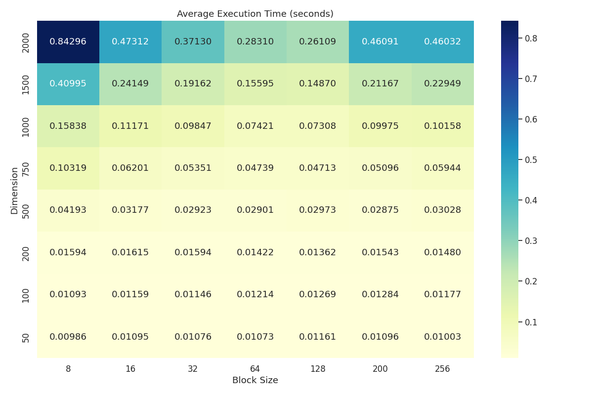
Execution Time Heatmap: Displays average execution time (seconds) with respect to matrix dimensions and block size for MULTITHREAD_9AVX.
As with MULTITHREAD_3AVX, we observe that block size 64 and 128 has the lowest mean for dimensions \(\delta=2000\) and \(\delta=1500\). We further verify that the mean for lower dimensions is relatively good as well. We perform the two-sided Welch's t-test and get the following plot.
As observed with MULTITHREAD_3AVX, block sizes 64 and 128 exhibit the lowest mean execution times for dimensions \(\delta = 2000\) and \(\delta = 1500\). These two block sizes also perform relatively well for lower dimensions. To further evaluate their performance, we utilize a two-sided Welch's t-test, which gives us the following plot.
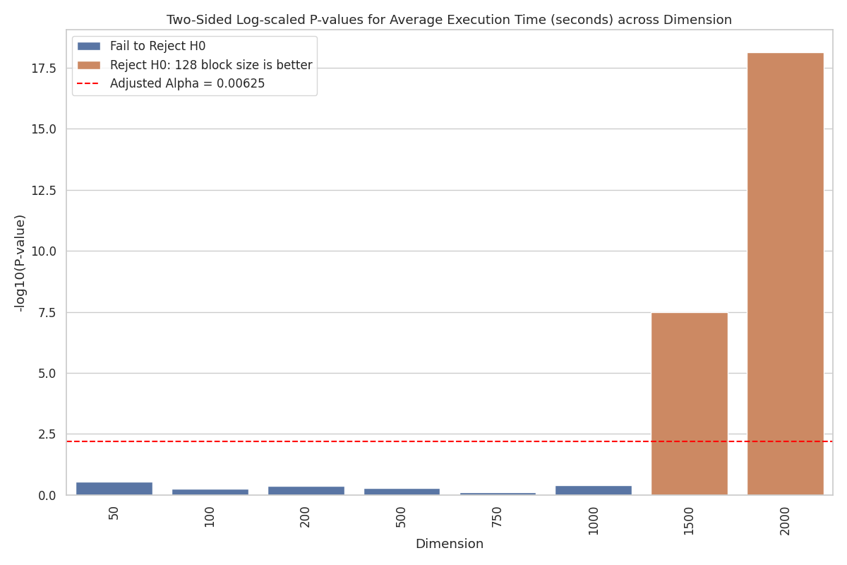
Rejection Threshold Plot: This plot visualizes p-values transformed as \(-\log_{10}(\text{P-value})\) for easier interpretation, and hypothesis rejection outcomes for MULTITHREAD_9AVX across different dimensions. Each bar corresponds to a specific dimension and represents its p-value. The red dotted line marks the adjusted alpha significance threshold (after Bonferroni correction). Brown bars indicates the rejection of \(H_{0}\) and that block size 128 has a smaller mean execution time than block size 64. Blue bars indicate failure to reject \(H_{0}\).
Inspecting the plot, the data provide evidence to reject \(H_0\) for \(\delta = 1500\) and \(\delta = 2000\). The heatmap confirms that block size 128 has a lower mean execution time for these dimensions. For the remaining dimensions, \(H_0\) is not rejected, indicating no statistically significant difference between the two block sizes at these levels.
In conclusion, the t-test results indicate a significant performance advantage for block size 128 at the two largest dimensions. Based on these findings, block size 128 is selected as the optimal block size for MULTITHREAD_9AVX.
1.4 Selection of the Best Algorithm
When incorporating SIMD vectorization, it was unclear whether utilizing three or nine (256-bit) AVX registers would yield better performance. Intuition suggested that adding more registers would lead to greater computational power, yet experimental data and analysis were needed to draw a conclusive result.
In the previous section, experiments and statistical analysis tests were conducted to determine the optimal block sizes for the algorithms: MULTITHREAD_3AVX and MULTITHREAD_9AVX. The results showed strong evidence that block size 128 outperformed block size 64 at higher matrix dimensions. For smaller dimensions, no significant difference was observed between the two block sizes. Based on these findings, block size 128 was selected as the optimal parameter for both algorithms.
This section determines the better-performing algorithm between MULTITHREAD_3AVX and MULTITHREAD_9AVX by analyzing the captured data from benchmarkresults.csv where a block size of 128 was applied. The following heatmap illustrates the average execution time for the algorithms over different dimensions.
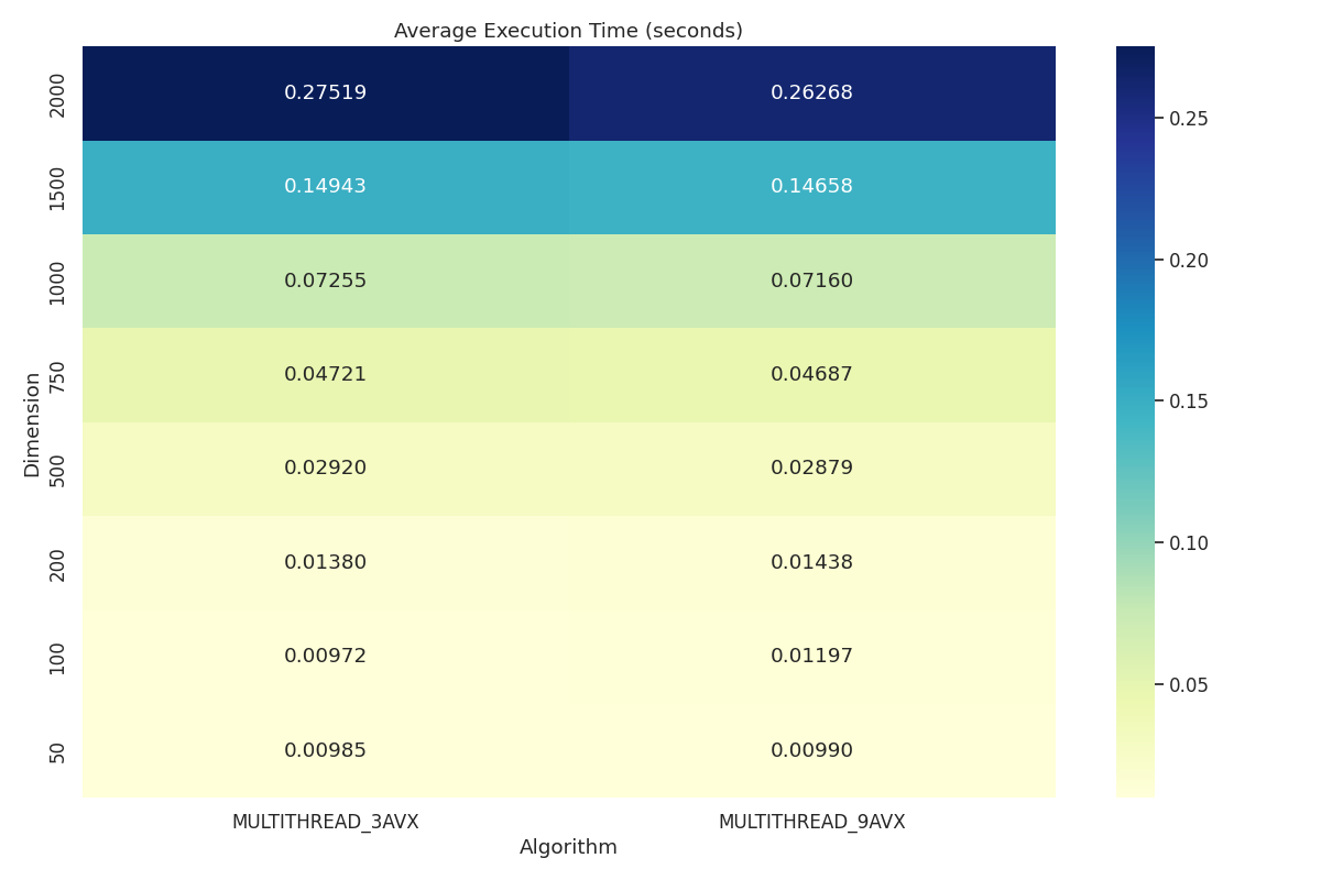
Execution Time Heatmap: Displays average execution time (seconds) with respect to matrix dimensions and competing algorithms: MULTITHREAD_3AVX and MULTITHREAD_9AVX.
For \(\delta=50\), \(\delta=100\) and \(\delta=200\), we observe that MULTITHREAD_3AVX has a slightly lower mean. For the higher dimensions, MULTITHREAD_9AVX has the lowest mean, with the largest difference occurring at \(\delta=2000\). To determine whether these differences in mean time are statistically significant, we apply Welch's two sided t-test with a Bonferroni correction of the alpha to reduce the risk of type I errors (false positives).
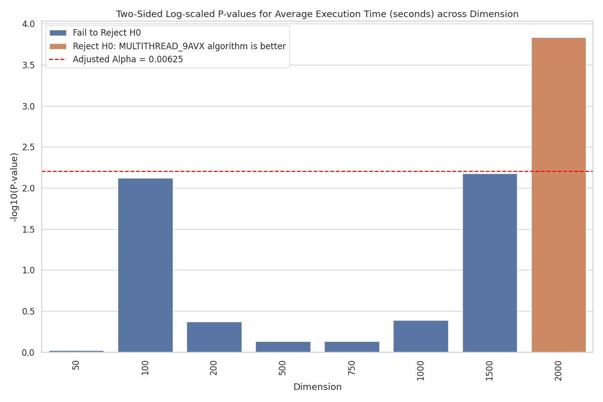
Welch's t-test Rejection Bar Plot: Illustrates p-values and null hypothesis rejections for competing algorithms: MULTITHREAD_3AVX, MULTITHREAD_9AVX. Each bar displays the p-value corresponding to each dimension. The red dotted line represents the adjusted alpha significant threshold (Bonferroni correction). If the null hypothesis is rejected, a brown colored bar indicates the mean execution time for MULTITHREAD_9AVX is smaller.
As initially observed in the heatmap, for \(\delta = 2000\), the data shows strong evidence that
MULTITHREAD_9AVX achieves a better runtime. For \(\delta = 1500\), the p-value is close to statistical significance, also favoring MULTITHREAD_9AVX. However, for \(\delta = 100\), the test nearly rejects the null hypothesis in favor of MULTITHREAD_3AVX.
Further data collection and testing might clarify whether the smaller mean for MULTITHREAD_3AVX observed in the heatmap is due to the algorithm being better suited for smaller dimensions, or whether it is simply a result of noise, variance, or randomness in the hardware across runs. Further testing
with higher dimensions would also be interesting, as it would help determine whether the performance gap observed in MULTITHREAD_9AVX for \(\delta = 2000\) continues to improve as the matrix size increases.
Nevertheless, Welch’s t-test reveals strong evidence of a difference for \(\delta = 2000\). Therefore, we accept MULTITHREAD_9AVX as the overall better-performing algorithm.
1.5 Benchmarking Algorithms
This section contains figures of the benchmark data found in benchmarkresults.csv for all the implemented algorithms and OpenBLAS. The purpose of the section is to highlight the iterative improvement between the implemented algorithms.
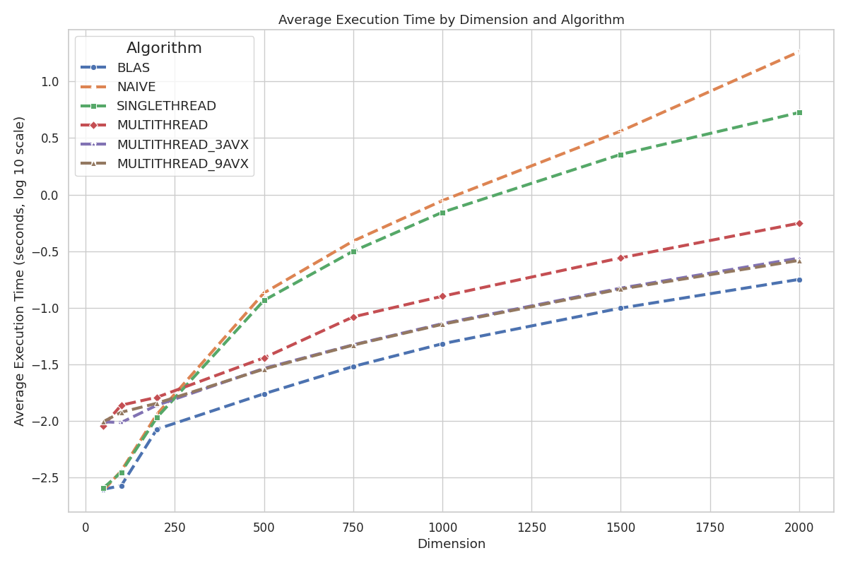
Execution Time Plot: Displays average execution time (seconds) of the implemented algorithms and OpenBLAS with respect to matrix dimensions.
Notice how the implemented algorithms NAIVE and SINGLETHREAD have a smaller mean execution time in the lower dimensions compared to the multithreaded algorithms. This difference is likely due to the overhead introduced by multithreading—such as thread initialization, mutex and queue interactions, and thread clean-up. Nevertheless, as the dimension increases, this overhead becomes negligible.
Further speculation suggests that OpenBLAS may utilize a single-threaded framework for the smallest dimensions, as its mean execution time closely matches that of NAIVE and SINGLETHREAD.
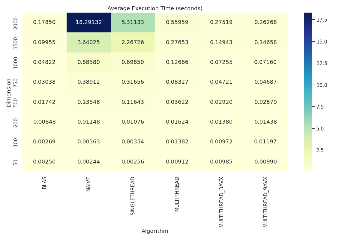
Execution Time Heatmap: Displays average execution time (seconds) of the implemented algorithms and OpenBLAS with respect to matrix dimensions.
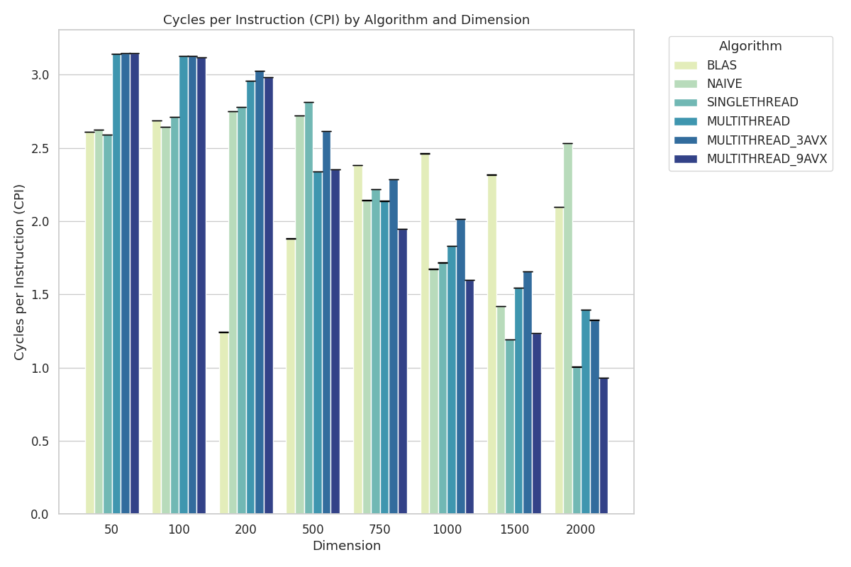
CPI Bar Chart: Displays cycles per instruction (CPI) of the implemented algorithms and OpenBLAS with respect to matrix dimensions.
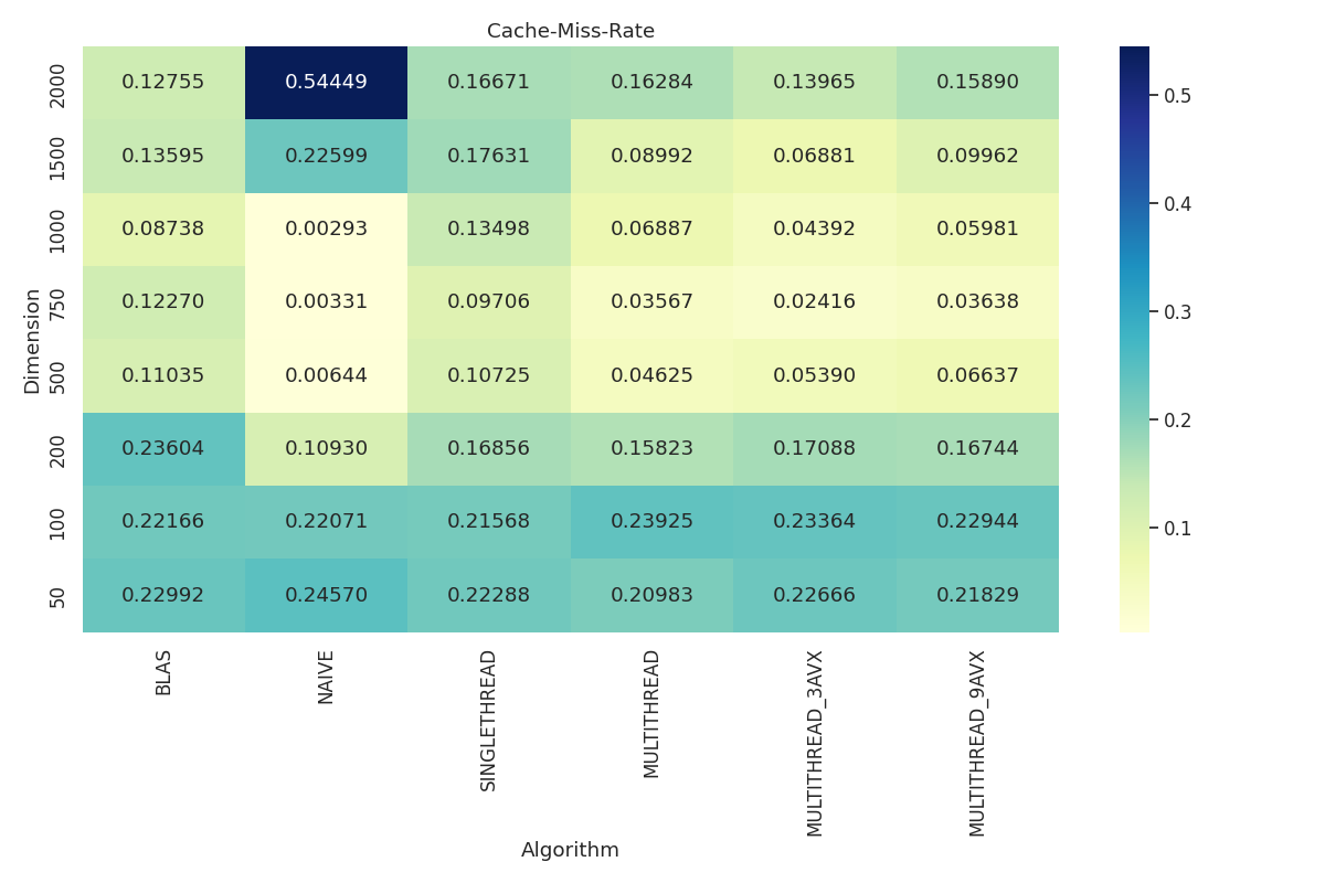
Cache-Miss Rate Heatmap: Displays cache-miss rate of the implemented algorithms and OpenBLAS with respect to matrix dimensions.
1.7 Conclusion
This project has served as a valuable milestone in learning low-level programming in C, demonstrating the iterative process of optimizing matrix multiplication algorithms, starting with the simple naive implementation. By implementing the blocking method, incorporating multithreading, and utilizing SIMD vectorization, a steady improvement in performance has been observed.
In addition, thorough benchmarking and statistical testing provided strong evidence that MULTITHREAD_9AVX outperforms MULTITHREAD_3AVX at higher matrix dimensions. As no statistically significant difference was found at lower dimensions, MULTITHREAD_9AVX is accepted as the best-performing algorithm overall
2. Appendix: Theory
This section provides detailed explanations of the algorithms developed throughout this project.
2.1 Naive Matrix Multiplication Algorithm - NAIVE
Our starting point is the naive matrix multiplication algorithm, which we will refer to as NAIVE. This implementation serves as the baseline from which we can improve to create better-performing algorithms.
For NAIVE, we use a triple-nested loop to perform matrix multiplication. For matrices \(A\) of size \(n \times m\) and \(B\) of size \(m \times p\), the resulting matrix \(C\) of size \(n \times p\) is computed by iterating over each element \(c_{ij}\) in \(C\). Iterating over \(c_{ij}\) is handled by the two outer loops seen in the pseudocode below. In the inner-most loop, we calculate each \(c_{ij}\). This is done by calculating the dot product of the \(i\)-th row of \(A\) and the \(j\)-th column of \(B\).
void matrix_mult_naive(Matrix* A, Matrix* B, Matrix* C) {

    /*
    * Logic for ensuring valid Matrix pointers and that
    * they are compatible for multiplication.
    */
    // ...

    // Retrieve internal Matrix arrays
    double* A_arr = A->values;
    double* B_arr = B->values;
    double* C_arr = C->values;

    // Extract Matrix dimensions
    size_t n = A->num_rows;
    size_t m = A->num_cols;
    size_t p = B->num_cols;

    for (size_t i = 0; i < n; i++) {
        for (size_t j = 0; j < p; j++) {

            // Calculate the dot product for this cell in Matrix C
            for (size_t k = 0; k < m; k++) {
                C_arr[i * p + j] += A_arr[i * m + k] * B_arr[k * p + j];
            }
        }
    }
}
2.1.1 Matrix Struct and One-Dimensional Arrays
To represent a matrix, we use the custom Matrix struct, which internally utilizes a one-dimensional array to represent a two-dimensional matrix. The struct contains member variables for the number of rows and columns, along with a member variable for the internal one-dimensional array. The number of rows and columns are needed to correctly index the one-dimensional array.
The benefits of a one-dimensional array are that all elements are stored contiguously in memory, which improves spatial locality. When a byte is accessed from memory by the CPU, the CPU fetches the whole corresponding cache line, not just the byte. This mechanism is in place because programs tend to work with adjacent bytes, like with an array for example. Thus, retrieving the entire cache line reduces multiple independent retrievals. This results in fewer cache misses and more efficient data retrieval.
To highlight further, a two-dimensional array (or an array of pointers) does not guarantee that rows are stored adjacently in memory like with a one-dimensional array. Each row could be allocated separately by the memory allocator, which may cause logically adjacent rows to be physically distant in memory. This worsens spatial locality, as potentially more cache lines need to be fetched by the CPU, increasing the likelihood of cache misses and inefficient use of the CPU caches.
2.1.2 Considerations
While the NAIVE algorithm is simple and easy to understand, it has several drawbacks, especially when dealing with large matrices.
- Inefficient Cache Usage With Large Matrix Sizes: To compute element \(c_{ij}\) from \(C\) in the inner-most loop, the algorithm accesses the entire \(i\)-th row of \(A\) and the entire \(j\)-th column of \(B\). For large matrices, these rows and columns may not fit within the CPU caches. As a result, the cache can become filled with data that might not be reused before being discarded, leading to cache misses. This causes the CPU to fetch data from memory more frequently, which slows down the computation since accessing memory is significantly slower than accessing data from the cache.
- Poor Spatial Locality When Accessing Columns of \(B\):
NAIVEaccesses the elements of \(B\) column-wise (i.e., \(B_{kj}\)), but since \(B\) is stored in row-major order in a one-dimensional array, its columns are not stored contiguously in memory. In the inner-most loop, we calculate each element \(c_{ij}\) by summing over the elements of row \(i\) in \(A\) multiplied with the elements of column \(j\) in \(B\) pairwise. When accessingA_arr, we efficiently retrieve adjacent elements due to the contiguous memory layout of \(A\). However, when accessingB_arr, we perform jumps in memory because \(B\)'s columns are not stored contiguously. This worsens spatial locality and may increase cache misses since each access to a new element in the column may require loading a new cache line. Thus, if the matrix is large, we may end up discarding already fetched cache lines, and thus not making the best use of data that we retrieve from memory. By transposing matrix \(B\), we convert the column-wise access into row-wise access, making the memory accesses contiguous and improving spatial locality.
2.2 Blocking / Tiling Method - SINGLETHREAD
The algorithm extending NAIVE by incorporating the blocking method and pre-transposing matrix \(B\) is referred to as SINGLETHREAD. The blocking method improves cache utilization by dividing the matrices into smaller submatrices (blocks) that fit into the CPU cache and be processed independently. For each block in \(C\), the corresponding rows of matrix \(A\) and columns of matrix \(B\) are partitioned into smaller blocks, which are then loaded into the CPU cache for efficient computation.
Transposing matrix \(B\), as mentioned in the previous section turns column-wise access into row-wise access, thus accessing contiguous data in memory.
The following is pseudocode for SINGLETHREAD. In the original code, loop unrolling is applied to further optimize performance along with variables containing precomputed values. This is not present in the pseudocode to maintain simplicity.
void matrix_singlethread_mult(Matrix* A, Matrix* B, Matrix* C, size_t block_size) {

    /*
    * Logic for ensuring valid Matrix pointers and that
    * they are compatible for multiplication.
    * Verify block_size is greater than 0.
    * Adjust block_size if it is larger than the smallest dimension
    * of all matrices to the smallest dimension.
    */
    // ...

    /*
    * Transpose the internal array of Matrix B to increase
    * spatial locality.
    */
    // B_trans_arr = ...;

    // Retrieve internal Matrix arrays
    double* A_arr = A->values;
    double* C_arr = C->values;

    // Extract Matrix dimensions
    size_t n = A->num_rows;
    size_t m = A->num_cols;
    size_t p = B->num_cols;

    // Iterate over blocks within the C matrix
    for (size_t i = 0; i < n; i += block_size) {
        for (size_t j = 0; j < p; j += block_size) {

            /*
            * Iterate over blocks in the shared dimension
            * (rows of A and columns of B) corresponding to
            * the current block in C.
            */
            for (size_t k = 0; k < m; k += block_size) {

                /*
                * We calculate i_max, j_max, and k_max to handle cases
                * where the block size does not divide the matrix
                * dimensions evenly. This ensures we don't access
                * out-of-bounds memory when processing the edge blocks.
                */
                size_t i_max = min(i + block_size, n);
                size_t j_max = min(j + block_size, p);
                size_t k_max = min(k + block_size, m);

                // Iterate over elements within the current block of C
                for (size_t ii = i; ii < i_max; ii++) {
                    for (size_t jj = j; jj < j_max; jj++) {

                        /*
                        * Update c_{ij} within the C block. Note that it is not
                        * fully calculated as this happens after we have gone
                        * through every block in the shared dimension k.
                        */
                        for (size_t kk = k; kk < k_max; kk++) {
                            C_arr[ii * p + jj] += A_arr[ii * m + kk] * B_trans_arr[jj * m + kk];
                        }
                    }
                }
            }
        }
    }
    // Free the helper B transpose array
    free(B_trans_arr);
}
By applying the SINGLETHREAD method, we address the inefficiencies of the NAIVE implementation related to cache usage and memory access patterns. The result is improved performance, especially for large matrices.
2.2.1 Considerations
With the blocking method, a block size parameter is introduced to determinine the size of the blocks. Finding an optimal parameter value is crucial for maximizing the algorithm's efficiency.
When the block size is set lower than optimal, several issues can arise. Smaller block sizes result in more blocks, which increases loop iterations and adds function overhead. Additionally, smaller blocks can lead to poorer cache utilization, particularly for matrix \(B\), as discussed in the NAIVE section. While the blocking method aims to optimize cache usage, smaller block sizes may underutilize cache lines.
In the NAIVE approach, retrieving a cache line often meant using only a single double before "jumping" to the next row of matrix \(B\). The blocking method improves this by allowing multiple contiguous doubles from the same cache line to be used before moving to the next row, thus better leveraging the CPU cache.
2.3 Multithreading - MULTITHREAD
The next improvement is the introduction of MULTITHREAD, an algorithm that builds upon SINGLETHREAD by utilizing multithreading to leverage multiple CPU cores in parallel. Multithreading integrates well with SINGLETHREAD and its blocking method, as each block of the result matrix \(C\) can be computed independently, without interfering with other blocks. The main change in MULTITHREAD is the refactoring of SINGLETHREAD to distribute tasks across multiple threads. To achieve this, two key components are introduced: the Task and the Queue struct.
The Task struct is a simple abstraction that encapsulates a unit of work for a thread. Each task contains member variables that define the specific block of \(C\) to be computed, including relevant indices and pointers to the matrices involved. By encapsulating the data required for each block calculation, we can distribute tasks among threads efficiently.
The Queue struct stores all tasks to be executed and ensures threads can retrieve tasks efficiently during runtime. To synchronize access to the shared queue, a mutex (mutual exclusion lock) is used. A mutex ensures that only one thread can access the queue at a time, preventing race conditions that could lead to incorrect computations or corrupted data.
The following two codeboxes provide pseudocode for matrix_multithread_mult and process_tasks. To maintain clarity, certain implementation details have been simplified in the pseudocode.
The first codebox, matrix_multithread_mult, represents the main function managing the multithreading. It handles the construction of tasks and the queue, initializing threads, assigning each thread the process_tasks function, and performing cleanup.
void matrix_multithread_mult(Matrix* A, Matrix* B, Matrix* C, size_t block_size, size_t NUM_THREADS) {

    /*
    * Validate Matrix pointers and ensure they are compatible for multiplication.
    * Verify block_size is greater than 0.
    */
    // ...

    // Extract Matrix dimensions
    size_t n = A->num_rows;
    size_t m = A->num_cols;
    size_t p = B->num_cols;

    // Create a Queue of tasks for computing blocks of Matrix C
    Queue* q = preprocessing(A, B, C, block_size);

    // Initialize the mutex for the threads to safely interact with the Queue
    pthread_mutex_init(&queue_lock, NULL);

    // Create an array of threads
    pthread_t threads[NUM_THREADS];

    // Assign threads the process_tasks function
    for (size_t i = 0; i < NUM_THREADS; i++) {
        pthread_create(&threads[i], NULL, process_tasks, q);
    }

    // Wait for all threads to complete
    for (size_t i = 0; i < NUM_THREADS; i++) {
        pthread_join(threads[i], NULL);
    }

    // Clean up resources
    queue_free(q);
    pthread_mutex_destroy(&queue_lock);
}
The second codebox, process_tasks, contains code executed by the threads. The code handles safe interaction with the queue. If its non-empty, the thread retrieves a task and uses thread_mult to perform the matrix multiplication for the specified block in \(C\). The matrix multiplication logic in thread_mult remains mostly unchanged from the previous implementation and is therefore not included here. The key difference is the removal of the two outer loops that dissect matrix \(C\) into blocks (see the pseudocode in section Blocking / Tiling Method - SINGLETHREAD). This is because information about the block is now stored in the Task struct.
void* process_tasks(void* arg) {

    Queue* q = (Queue*) arg;

    while (true) {
        Task t;
        bool is_empty;

        // Lock the mutex before accessing the Queue
        pthread_mutex_lock(&queue_lock);

        /*
        * The thread interacts with the Queue. To minimize
        * time spent occupying the mutex, the thread simply
        * retrieves a Task if the Queue is non-empty.
        * All other processing happens after unlocking the mutex,
        * allowing other threads to interact with the Queue.
        */
        is_empty = queue_is_empty(q);
        if (!is_empty) {
            t = queue_get(q);
        }

        // Unlock the mutex
        pthread_mutex_unlock(&queue_lock);

        // If the Queue is empty, exit the loop
        if (is_empty) {
            break;
        }

        // Perform matrix multiplication for the current Task
        thread_mult(t);
    }

    return NULL;
}
2.3.1 Considerations
When using multithreading, it is important to balance the introduced overhead from thread creation and management with the performance benefits. For small matrices, this overhead can outweigh the advantages of parallel computation, making multithreading less effective.
Additionally, selecting an optimal block size parameter is crucial. A block size that creates very small submatrices increases the number of tasks, which in turn increases the ratio of overhead to actual computation, as more time is spent setting up tasks and managing threads relative to performing matrix multiplications.
2.4 SIMD Vectorization - MULTITHREAD_3AVX, MULTITHREAD_9AVX
As a final optimization step, we introduce AVX vectorization to perform calculations in parallel within the CPU. In standard operations, a CPU register typically holds a single value, such as a double, and operates on it individually. An AVX register, however, can hold multiple values simultaneously (depending on their size) and perform operations on all of them in parallel. This can greatly enhance the performance of compute-intensive tasks like matrix multiplication.
To perform the matrix multiplications using AVX registers (256 bytes), a total of three registers are used. This is reflected in the names of this section's algorithms: MULTITHREAD_3AVX and MULTITHREAD_9AVX. The former algorithm uses three AVX registers, the smallest number of registers needed to perform the matrix multiplication. The latter algorithm uses nine AVX registers. Internally, this algorithm represents the scaling of the matrix code by a factor of three.
void thread_mult_3avx(Task t) {

    // Retrieve matrices: A x B = C
    Matrix* A = t.A;
    Matrix* B_trans = t.B_trans;
    Matrix* C = t.C;

    // Extract Matrix dimensions
    size_t m = A->num_cols;
    size_t p = B_trans->num_rows;

    // Retrieve internal Matrix arrays
    double* A_arr = A->values;
    double* B_trans_arr = B_trans->values;
    double* C_arr = C->values;

    // The block size to use (blocking method)
    size_t block_size = t.block_size;

    // Variables to describe the C block (start inclusive, end exclusive)
    size_t C_row_start = t.C_row_start;
    size_t C_col_start = t.C_col_start;
    size_t C_row_end = t.C_row_end;
    size_t C_col_end = t.C_col_end;

    // Loop goes through blocks in the shared dimension
    for (size_t k = 0; k < m; k += block_size) {
        // Makes sure we stay within the block and shared matrix dimension
        size_t k_min = min(k + block_size, m);

        // The two following loops goes through all elements c_{ij} in the block
        for (size_t ii = C_row_start; ii < C_row_end; ii++) {
            // Precomputed variable
            size_t a_row_offset = ii * m;
            for (size_t jj = C_col_start; jj < C_col_end; jj++) {

                // Precomputed variables
                size_t kk = k;
                size_t c_index = ii * p + jj;
                size_t b_row_offset = jj * m;
                double c_value = C_arr[c_index];

                /*
                 * Using AVX (256 bytes) registers to speed up the process (SIMD).
                 * The implementation below follows these steps:
                 * 1. Initialize the first AVX register to 0 (c_vec).
                 * 2. Load 4 doubles from A into the second AVX register.
                 * 3. Load 4 doubles from B into the third AVX register.
                 * 4. Perform the multiplication and add the value to c_vec.
                 * 5. Unwrap the c_vec value using an array.
                 * 6. Add the elements of c_vec into a single value.
                 */

                // Initialize AVX register to zero. These will act as a holder
                // containing the accumulation of the dot product for a single
                // (ii,jj) cell in C when going over the block corresponding
                // to k.
                __m256d c_vec = _mm256_setzero_pd();
                for (; kk + 3 < k_min; kk += 4) {

                    // Load the 4 doubles from A starting from the address given
                    // as function argument.
                    __m256d a_vals = _mm256_loadu_pd(&A_arr[a_row_offset + kk]);

                    // Load the 4 doubles from B starting from the address given
                    // as function argument.
                    __m256d b_vals = _mm256_loadu_pd(&B_trans_arr[b_row_offset + kk]);

                    // Multiply the dot product between the A and B values
                    // in the AVX registers and add the value to the
                    // c_vec.
                    c_vec = _mm256_fmadd_pd(a_vals, b_vals, c_vec);
                }

                // Unwrap the c_vec and sum up the elements in the vector
                double temp[4];
                _mm256_store_pd(temp, c_vec);
                c_value += temp[0] + temp[1] + temp[2] + temp[3];

                // Handle residual operations not handled by the SIMD loop
                for (; kk < k_min; kk++) {
                    c_value += A_arr[a_row_offset + kk] * B_trans_arr[b_row_offset + kk];
                }

                // Write back to memory
                C_arr[c_index] = c_value;
            }
        }
    }
}
